
Deep neural networks are currently used by companies such as Facebook, Google, Apple, etc. for making predictions from massive amounts of user generated data. A few examples are the Deep Face and Deep Text systems used by Facebook for face recognition and text understanding or the speech recognition systems used by Siri and Google Now. In this type of applications, it is critical to use neural networks that make predictions that are both fast and accurate. This means that, when designing these systems, we would like to tune different neural network parameters to jointly minimize two objectives: 1) the prediction error on some validation data and 2) the prediction speed. The parameters to tune, also called the design parameters, could be the number of hidden layers, the number of neurons per layer, learning rates, regularization parameters, etc.
Minimizing the prediction error and the prediction speed involves solving a multi-objective optimization problem. In this type of problems, in general, there is no single optimal solution that jointly minimizes the different objectives. Instead, there is a collection of optimal solutions called the Pareto front.
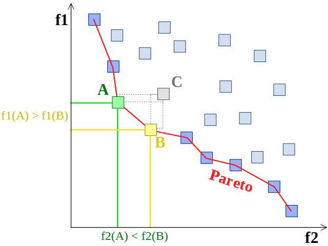
Example of Pareto front. Each point in the plot shows the objective values (f1 and f2) obtained for a particular setting of the design parameters. The points highlighted in blue are in the Pareto front.
The points in the Pareto front attain an optimal trade-off between objectives in the sense that you cannot move from one point in the Pareto front to another arbitrary point by improving one of the objectives without deteriorating the other. The figure above shows an example of a Pareto front for two objectives f1 and f2. Each point in the plot shows the objective values obtained for a particular choice of the design parameters. When solving a multi-objective optimization problem we are interested in finding values of the design parameters that map to points in the Pareto front. Once we have found the points in the Pareto front, we can make a decision and choose one that satisfies our requirements.
In the neural network tuning problem, the evaluation of the prediction error for a particular setting of the design parameters is a computationally expensive process. The reason for this is that, before being able to compute the validation error, we have to first train the neural network on large amounts of training data. With large neural networks and massive datasets this process can take many hours or even days. This means that, ideally, we would like to find the Pareto front using a small number of objective evaluations. This can be done by using Bayesian optimization (BO) techniques. These methods use the predictions of a model to efficiently search for the solution of expensive optimization problems. In this post, I will describe how to use the BO method Predictive Entropy Search for Multi-objective Optimization (PESMO)
Hernández-Lobato D., Hernández-Lobato J. M., Shah A. and R. P. Adams.
Predictive Entropy Search for Multi-objective Bayesian Optimization,
In ICML, 2016. [pdf] [Spearmint code]
for finding deep neural networks with optimal prediction error vs. prediction speed on the MNIST dataset. PESMO is the current state-of-the-art technique for multi-objective optimization with expensive objective functions. For more information about BO methods the reader can have a look at [1,2].
Finding networks that produce fast and accurate predictions on MNIST
PESMO is implemented in the PESM branch of the spearmint tool, which is publicly available at the link shown above. After installing the PESM branch of spearmint in our system, we have to specify the multi-objective optimization problem that we want to solve. In our case, we will be tuning the following design parameters in our neural networks:
- The number of hidden layers.
- The number of neurons per hidden layer.
- The level of dropout.
- The learning rate to use with the ADAM optimizer [3].
- The L1 weight penalty.
- The L2 weight penalty.
This information is provided to spearmint in a file called config.json, which contains details of the optimization problem such as the variables to be tuned, their maximum and minimum values, how many objectives we will be optimizing, how to evaluate the objectives, etc. We will be using the following config.json file:
    {
    "language"        : "PYTHON",
    "random_seed"     : 1,
    "grid_size"       : 1000,
    "max_finished_jobs"       : 100,
    "experiment-name" : "MNIST_neural_networks",
    "moo_use_grid_only_to_solve_problem" : true,
    "moo_grid_size_to_solve_problem" : 1000,
    "pesm_use_grid_only_to_solve_problem" : true,
    "likelihood"      : "GAUSSIAN",
    "acquisition"     : "PESM",
    "pesm_pareto_set_size"      : 50,
    "pesm_not_constrain_predictions"     : false,
    "main_file"       : "evaluate_objectives",
    "variables": {
        "n_neurons": {
            "type": "FLOAT",
            "size":  1,
            "min":  50,
            "max":  500
        }, "n_hidden_layers": {
            "type": "FLOAT",
            "size": 1,
            "min":  1,
            "max":  3
        }, "prob_drop_out": {
            "type": "FLOAT",
            "size": 1,
            "min":  0,
            "max":  0.9
        }, "log_learning_rate": {
            "type": "FLOAT",
            "size": 1,
            "min": -20,
            "max":  0
        }, "log_l1_weight_reg": {
            "type": "FLOAT",
            "size": 1,
            "min": -20,
            "max":  0
        }, "log_l2_weight_reg": {
            "type": "FLOAT",
            "size": 1,
            "min": -20,
            "max":  0
        }
    },
    "tasks": {
      "error_task" : {
          "type"        : "OBJECTIVE",
          "fit_mean"    : false,
          "transformations"     : [],
          "group"    : 0
      },
      "time_task" : {
          "type"        : "OBJECTIVE",
          "transformations" : [
                {"IgnoreDims" : { "to_ignore" : [ 2, 3, 4, 5 ]   }}
                ],
          "fit_mean"    : false,
          "group"    : 0
      }
    }
}
|
I will describe a few important entries in this file. The entry main_file contains the name of a python script that will be called to evaluate the different objectives. The entry max_finished_jobs takes value 100. This indicates spearmint to evaluate the different objectives 100 times and then finish. The entry variables contains a description of the design parameters, with their maximum and minimum values. The entry tasks contains a description of the objectives to be optimized. Note that the prediction time does not depend on the parameters dropout, learning rate, L1 penalty and L2 penalty. We inform spearmint of this by using the entry IgnoreDims in the transformations of the objective for the prediction time objective.
The next step is to write the python script that will evaluate the different objectives. We have already told spearmint that this file is called evaluate_objectives.py, which contains the following code based on Keras [4]:
import numpy as np
import time
from keras.datasets import mnist
from keras.models import Sequential
from keras.layers.core import Dense, Dropout, Activation
from keras.optimizers import Adam
from keras.utils import np_utils
from keras.regularizers import l1l2, l2, activity_l2

def build_model(params):

    n_hidden_layers = int(np.round(params['n_hidden_layers'][ 0 ]))
    n_neurons = int(np.round(params['n_neurons'][ 0 ]))
    log_l1_weight_reg = params['log_l1_weight_reg'][ 0 ]
    log_l2_weight_reg = params['log_l2_weight_reg'][ 0 ]
    prob_drop_out = float(params['prob_drop_out'][ 0 ].astype('float32'))
    log_l_rate = params['log_learning_rate'][ 0 ]

    model = Sequential()
    model.add(Dense(n_neurons, input_shape = (784,), W_regularizer=l1l2(l1 = np.exp(log_l1_weight_reg), \
        l2 = np.exp(log_l2_weight_reg))))
    model.add(Activation( 'relu'))
    model.add(Dropout(prob_drop_out))
    for i in range(n_hidden_layers - 1):
        model.add(Dense(n_neurons, W_regularizer=l1l2(l1 = np.exp(log_l1_weight_reg), \
            l2 = np.exp(log_l2_weight_reg))))
        model.add(Activation( 'relu'))
        model.add(Dropout(prob_drop_out))
    n_classes = 10
    model.add(Dense(n_classes))
    model.add(Activation( 'softmax'))
    adam = Adam(lr=np.exp(log_l_rate), beta_1=0.9, beta_2=0.999, epsilon=1e-08)
    model.compile(loss='categorical_crossentropy', optimizer=adam)

    return model

def evaluate_error_model(X_train, Y_train, X_test, Y_test, X_val, Y_val, params):

    nb_epoch = 150
    batch_size = 4000
    model = build_model(params)
    model.fit(X_train, Y_train, batch_size=batch_size, nb_epoch=nb_epoch, show_accuracy=True, verbose=2, \
        validation_data=(X_val, Y_val))
    loss, score = model.evaluate(X_val, Y_val, show_accuracy=True, verbose=0)
    print('Val error:', 1.0 - score)
    return np.log((1 - score) / score)

def evaluate_time_model(X_train, Y_train, X_test, Y_test, X_val, Y_val, params):

    nb_epoch = 1
    batch_size = 500
    model = build_model(params)
    start = time.time()
    for i in range(100):
        predictions = model.predict_classes(X_val, batch_size=X_val.shape[ 0 ], verbose=0)
    end = time.time()
    print('Avg. Prediction Time:', (end - start) / 100.0)
    return (end - start) / 100.0

def main(job_id, params):

    nb_classes = 10
    (X_train, y_train), (X_test, y_test) = mnist.load_data()
    X_train = X_train.reshape(60000, 784)
    X_test = X_test.reshape(10000, 784)
    X_train = X_train.astype('float32')
    X_test = X_test.astype('float32')
    X_train /= 255
    X_test /= 255

    state = np.random.get_state()
    np.random.seed(0)
    suffle = np.random.permutation(60000)
    i_train = suffle[ 0 : 50000 ]
    i_val = suffle[ 50000 : 60000 ]
    np.random.set_state(state)
    X_val = X_train[ i_val, : ]
    y_val = y_train[ i_val ]
    X_train = X_train[ i_train, : ]
    y_train = y_train[ i_train ]

    Y_train = np_utils.to_categorical(y_train, nb_classes)
    Y_test = np_utils.to_categorical(y_test, nb_classes)
    Y_val = np_utils.to_categorical(y_val, nb_classes)

    evaluation = dict()
    evaluation['error_task'] = evaluate_error_model(X_train, Y_train, X_test, Y_test, X_val, Y_val, params)
    evaluation['time_task'] = evaluate_time_model(X_train, Y_train, X_test, Y_test, X_val, Y_val, params)

    return evaluation
|
Note that in the function build_model we round to integers the variables n_neurons and n_hidden_layers, which are assumed to be continuous by spearmint. Also, in this script, the function evaluate_error_model returns the logit of the error and not the error itself. The logit transformation expands the range of variation of the error for values close to zero and will allow the Gaussian process models used by spearmint to better describe the collected data. Once we have finished writing the config.json and the evaluate_objectives.py files, we will use spearmint to solve the optimization problem. Let us assume that the current working directory contains the files config.json and evaluate_objectives.py. Then we run spearmint by typing
$ python /path_to_spearmint_folder/main.py . |
where path_to_spearmint_folder is the route to the folder where we have installed the PESM branch of spearmint. Spearmint will then evaluate the two objectives 100 times. After each of these evaluations, spearmint produces a recommendation with several points that are expected to be in the Pareto front. In general, the quality of these recommendations increases with the amount of data collected by spearmint. Therefore, in general, we will only be interested in the last of these recommendations. All the recommendations are stored by spearmint in a mongodb database. We can extract the last recommendation by using the python script extract_recommendations.py:
import os
import sys
import numpy as np

from spearmint.utils.parsing          import parse_config_file
from spearmint.utils.database.mongodb import MongoDB
from spearmint.tasks.input_space      import InputSpace

def main():

    options         = parse_config_file('.', 'config.json')
    experiment_name = options["experiment-name"]
    input_space     = InputSpace(options["variables"])
    db              = MongoDB(database_address=options['database']['address'])

    i = 0
    recommendation = db.load(experiment_name, 'recommendations', {'id' : i + 1})
    while recommendation is not None:
        params_last = input_space.vectorify(recommendation[ 'params' ])
        recommendation = db.load(experiment_name, 'recommendations', {'id' : i + 1})
        i += 1

    np.savetxt('pareto_front.txt', params_last, fmt = '%e')

if __name__ == '__main__':
    main()
|
We store this script in the same folder as the config.json file and execute it using
$ python extract_recommendations.py |
The script extract_recommendations.py stores the values of the design parameters that are estimated to be in the Pareto front in the file pareto_front.txt. We can then evaluate the objectives at the recommended points using the script evaluate_objectives.py and choose the one that best fits our requirements. The following figure shows the average Pareto front obtained with PESMO and with other existing BO methods over 50 repetitions of the optimization process. Overall, PESMO is able to find neural networks with better trade-offs between prediction accuracy and prediction speed than the alternative techniques. By visualizing the Pareto front, as shown in the figure, we can also make better decisions regarding which points from the Pareto front we would like to choose.
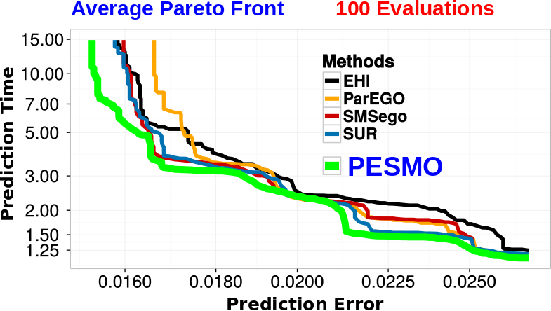
Comparison of PESMO with other BO techniques in the task of finding neural networks that make accurate and fast predictions on the MNIST dataset. Each axis represents a different objective and the curves show the Pareto front produced by each method. On average, the Pareto front recommended by PESMO dominates all the others.
Decoupled evaluations
In the previous example we have always evaluated the two objectives one after the other and at the same input location. However, in practice, these two functions can be evaluated in a decoupled way, that is, independently and at different locations. Note that, to evaluate the prediction error on the validation data, we have to train the neural network first. However, training is not necessary for evaluating the prediction time, which can be done using a neural network with arbitrary weight values. This allows us to decouple the evaluation of these two objectives. In this decoupled setting, at any given time we could choose to evaluate the prediction error or the prediction time. In general, considering an optimization problem with decoupled objectives as such can produce significant gains, especially when one of the objectives is expensive to evaluate and not very informative about the solution to the optimization problem. Interestingly, PESMO also allows for solving multi-objective optimization problems with decoupled objectives. More details about optimization problems with decoupled function evaluations can be found in the reference for PESMO shown above or in [5]. An example application of decoupled Bayesian optimization in the constrained setting is given in [6]. In this work Predictive Entropy Search with Constraints (PESC) [7] is used to optimize the accuracy a statistical machine translation system while ensuring that decoding speed exceeds a minimum value.
References
-
Brochu, Eric, Vlad M. Cora, and Nando De Freitas. A tutorial on Bayesian optimization of expensive cost functions, with application to active user modeling and hierarchical reinforcement learning, arXiv preprint arXiv:1012.2599 (2010).
-
Shahriari, Bobak, et al. Taking the human out of the loop: A review of Bayesian optimization, Proceedings of the IEEE 104.1 (2016): 148-175.
-
Kingma, Diederik, and Jimmy Ba. Adam: A method for stochastic optimization. arXiv preprint arXiv:1412.6980 (2014).
- http://keras.io
- Hernández Lobato J. M., Gelbart M. A., Adams R. P, Hoffman M. W. and Ghahramani Z. A General Framework for Constrained Bayesian Optimization using Information-based Search, Journal of Machine Learning Research, (in press), 2016. [pdf]
-
Daniel Beck, Adrià de Gispert, Gonzalo Iglesias, Aurelien Waite and Bill Byrne. Speed-Constrained Tuning for Statistical Machine Translation Using Bayesian Optimization. arXiv preprint arXiv:1604.05073 (2016).
- Hernández-Lobato J. M., Gelbart A. M., Hoffman M. W., Adams R. and Ghahramani Z. Predictive Entropy Search for Bayesian Optimization with Unknown Constraints, In ICML, 2015. [pdf] [supp. material] [python code]
